Neural Networks

Feedforward Neural Networks

A feedforward neural network is described by a directed acyclic graph, $G=$ $(V, E)$, and a weight function over the edges, $w: E \rightarrow \mathbb{R}$. Nodes of the graph correspond to neurons. Each single neuron is modeled as a simple scalar function, $\sigma: \mathbb{R} \rightarrow \mathbb{R}$. We will focus on three possible functions for $\sigma$ : the sign function, $\sigma(a)=\operatorname{sign}(a)$, the threshold function, $\sigma(a)=\mathbb{1}_{[a>0]}$, and the sigmoid function, $\sigma(a)=1 /(1+\exp (-a))$, which is a smooth approximation to the threshold function. We call $\sigma$ the "activation" function of the neuron. Each edge in the graph links the output of some neuron to the input of another neuron. The input of a neuron is obtained by taking a weighted sum of the outputs of all the neurons connected to it, where the weighting is according to $w$.

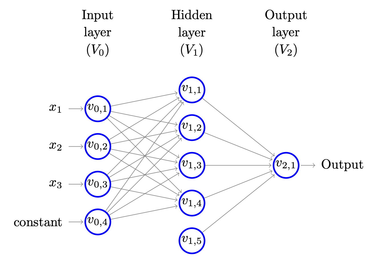
To simplify the description of the calculation performed by the network, we further assume that the network is organized in layers. That is, the set of nodes can be decomposed into a union of (nonempty) disjoint subsets, $V=\cup_{t=0}^T V_t$, such that every edge in $E$ connects some node in $V_{t-1}$ to some node in $V_t$, for some $t \in[T]$. The bottom layer, $V_0$, is called the input layer. It contains $n+1$ neurons, where $n$ is the dimensionality of the input space. For every $i \in[n]$, the output of neuron $i$ in $V_0$ is simply $x_i$. The last neuron in $V_0$ is the "constant" neuron, which always outputs 1 . We denote by $v_{t, i}$ the $i$ th neuron of the $t$ th layer and by $o_{t, i}(\mathbf{x})$ the output of $v_{t, i}$ when the network is fed with the input vector $\mathbf{x}$. Therefore, for $i \in[n]$ we have $o_{0, i}(\mathbf{x})=x_i$ and for $i=n+1$ we have $o_{0, i}(\mathbf{x})=1$. We now proceed with the calculation in a layer by layer manner. Suppose we have calculated the outputs of the neurons at layer $t$. Then, we can calculate the outputs of the neurons at layer $t+1$ as follows. Fix some $v_{t+1, j} \in V_{t+1}$. Let $a_{t+1, j}(\mathbf{x})$ denote the input to $v_{t+1, j}$ when the network is fed with the input vector $\mathbf{x}$. Then,

$$a_{t+1, j}(\mathbf{x})=\sum_{r:\left(v_{t, r}, v_{t+1, j}\right) \in E} w\left(\left(v_{t, r}, v_{t+1, j}\right)\right) o_{t, r}(\mathbf{x})$$

and

$$o_{t+1, j}(\mathbf{x})=\sigma\left(a_{t+1, j}(\mathbf{x})\right) .$$

That is, the input to $v_{t+1, j}$ is a weighted sum of the outputs of the neurons in $V_t$ that are connected to $v_{t+1, j}$, where weighting is according to $w$, and the output of $v_{t+1, j}$ is simply the application of the activation function $\sigma$ on its input. Layers $V_1, \ldots, V_{T-1}$ are often called hidden layers. The top layer, $V_T$, is called the output layer. In simple prediction problems the output layer contains a single neuron whose output is the output of the network.

We refer to $T$ as the number of layers in the network (excluding $V_0$ ), or the "depth" of the network. The size of the network is $|V|$. The "width" of the network is $\max _t\left|V_t\right|$. An illustration of a layered feedforward neural network of depth 2 , size 10 , and width 5 , is given in the following. Note that there is a neuron in the hidden layer that has no incoming edges. This neuron will output the constant $\sigma(0)$.

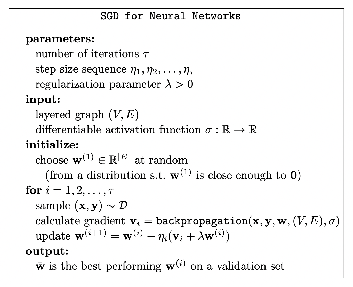
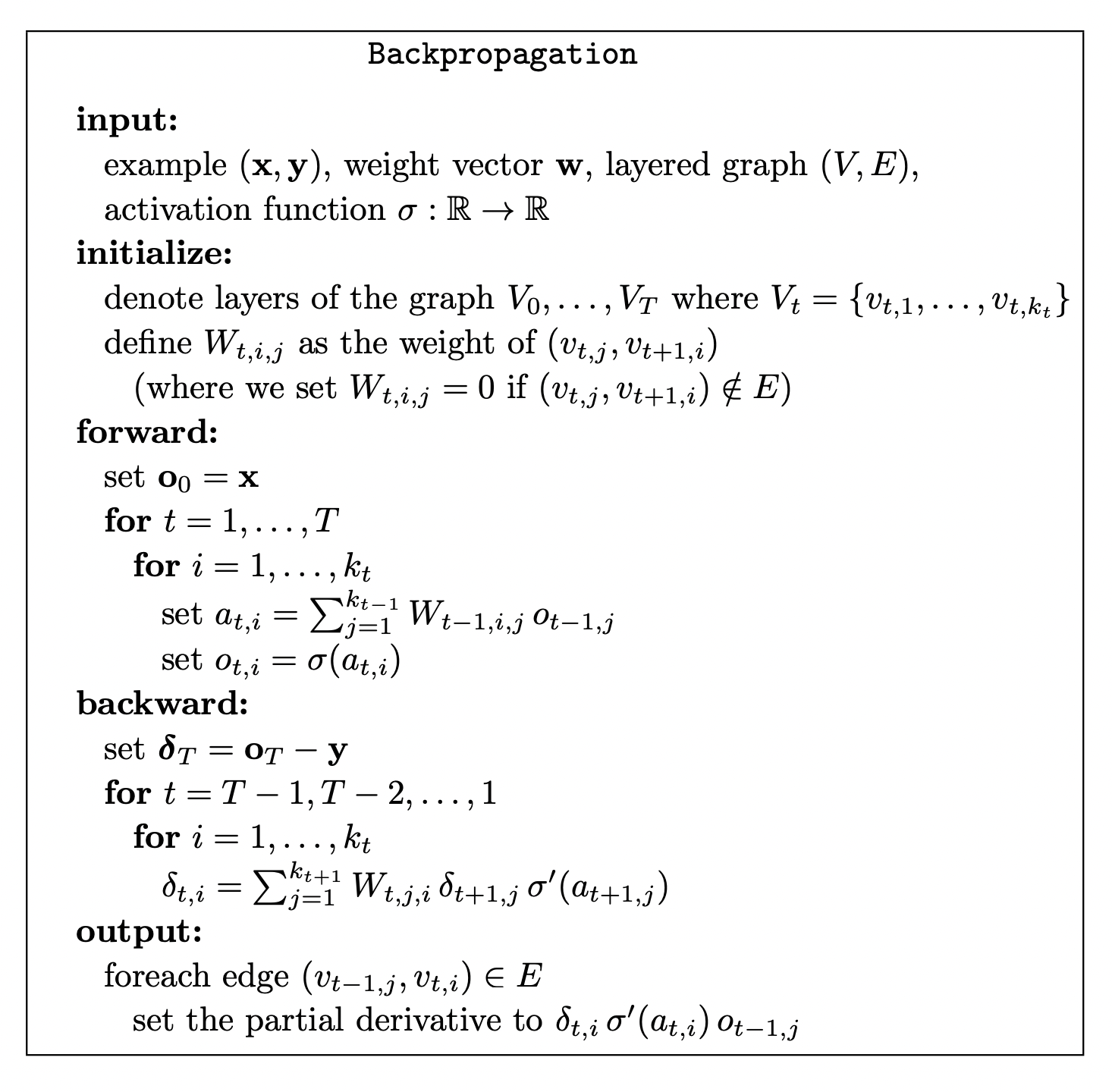
SGD and Backpropagation